Projects / Liveability index
Scoring inner Sydney with PostGIS
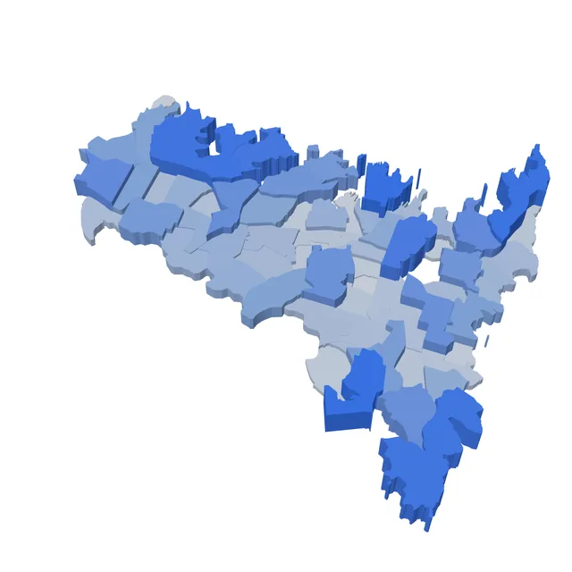
A database that pulls live NSW Government data, joins it to ABS statistical areas with spatial queries, and gives each of 66 SA2 regions a single liveability score between 0 and 1.
The question
If you only had public data, could you rank Sydney suburbs on how liveable they are, and could you defend the ranking? I scoped it to three ABS SA4 areas (Inner West, City and Inner South, Eastern Suburbs), which gives 66 SA2 regions. SA2 is the level the ABS publishes population at, so every other dataset had to be brought down to it.
Data in
- SA2 boundaries and population from the ABS, including total residents and young residents
- Transport stops pulled live from a NSW Government API with a Python collector: 5,870 stops in scope
- Businesses, schools and points of interest as point and count datasets: 3,204 points of interest in scope
Each source landed in its own table in a normalised schema, keyed by SA2 code where it had one and by geometry where it didn't.
Spatial joins
Most of the inputs are points. To count them per region I joined each point to the SA2 polygon that contains it. Normalising by population turns raw counts into something comparable between a dense inner suburb and a big low-density one.
-- map transport stops to SA2 boundaries, per 1,000 residents
SELECT sa2.sa2_code,
       sa2.sa2_name,
       COUNT(stop.stop_id) AS transport_stops,
       ROUND(COUNT(stop.stop_id)::numeric
             / NULLIF(pop.total_population, 0) * 1000, 2) AS stops_per_1000
FROM sa2_boundaries sa2
JOIN population_stats pop ON pop.sa2_code = sa2.sa2_code
LEFT JOIN transport_stops stop ON ST_Within(stop.geom, sa2.geom)
GROUP BY sa2.sa2_code, sa2.sa2_name, pop.total_population;

-- without this, every stop is tested against every polygon
CREATE INDEX idx_transport_geom ON transport_stops USING GIST (geom);
The GiST index is what makes the join usable. Without it PostGIS has to test every stop against every polygon. With it, it checks bounding boxes first and only runs the exact containment test on the few polygons that could match.
Turning four numbers into one
Each region ends up with four inputs: businesses per 1,000 residents in three industries (information and telecoms, transport and warehousing, manufacturing), the number of transport stops, school catchments per 1,000 young residents, and the number of points of interest. They're on completely different scales, so I converted each to a z-score, added the four together, and passed the sum through a logistic function to land between 0 and 1.
score = 1 / (1 + e-(z_business + z_stops + z_schools + z_poi))
Equal weights was a deliberate choice. I had no defensible reason to say transport matters twice as much as schools, so I didn't pretend to.
What came out
- Top: Millers Point, Banksmeadow, and Rose Bay - Vaucluse - Watsons Bay
- Bottom: Zetland, Pyrmont and Rhodes
- The median region scores 0.38, and 8 of 66 score above 0.9
- The Inner West is the most even, with the highest median (0.50) and the tightest spread. City and Inner South and the Eastern Suburbs are mostly low with a few extreme highs
What I'd change
Small populations break per-capita measures
Banksmeadow ranks second. It's mostly industrial land next to Port Botany with 507 residents, so its business and school measures get divided by a tiny number and its z-scores come out at 5.9 and 7.3. That's a denominator problem, not a liveable suburb. I'd set a minimum population, or shrink small regions towards the mean, before ranking anything.
The logistic squashes the top end
Millers Point has a z-sum of 11.5 and Banksmeadow 10.4, but both round to a score of 1.000. Rose Bay, at 4.1, gets 0.984. The logistic flattens out so fast that the index can't tell the top regions apart. Reporting percentile ranks, or the raw z-sum next to the score, would fix that.
The bottom of the list needs a second look
Pyrmont, Ultimo and Zetland are central and well served, and they sit near the bottom. I haven't pinned down why yet, so I wouldn't trust that end of the ranking until I have.
Not all inputs are normalised the same way
Stops and points of interest go in as counts, so bigger regions get a head start. I'd normalise everything by population or area, and show both versions.
If I ran this as a service
Right now it's a pipeline I run by hand. To keep it running unattended I'd:
- Schedule the collector and make loads idempotent, so a rerun can't double-count stops
- Track data freshness as the main SLI: how old is the newest row from the API
- Alert when the API's response shape changes or a load returns far fewer rows than last time
- Version each scoring run so a change to the formula never silently rewrites old results